NISOx: SwE

SwE: Manual

Sandwich Estimator Toolbox for Longitudinal & Repeated Measures Data

A toolbox for SPM

By Bryan Guillaume & Thomas Nichols

This page...

News

Introduction

Manual

FMRI worked example

Download

References

Contact

The goal of this manual is to explain how to use the SwE toolbox. If something is unclear or if you think more explanations are needed, please do not hesitate to contact Bryan Guillaume or Tom Nichols. The manual will be updated accordingly. Note that an example of the use of the toolbox on a real dataset can be found here. Note that this manual does not account for the new features of the last release of the toolbox. It will be updated soon.

Toolbox overview

The SwE toolbox implements the Sandwich Estimator (SwE) method described in Guillaume et al. (in submission) allowing the analysis of longitudinal and repeated measures data in neuroimaging. An analysis with the SwE toolbox can be decomposed into three stages:

Data & design setup (swe_design)
Computation of the model parameters (swe_cp)
Post-processing & display of results (swe_result_ui)

Each stage is handled by a separate function, callable either from the command line or the SwE GUI, as described below. Interim communication between the stages is done via SwE.mat files, similar to SPM.mat files. The setup stage (swe_design) launches the batch system and saves the configuration information in a SwE.mat. Note that the filenames of the input and created images are coded into the SwE.mat file, so moving or deleting the images may cause issues. The computation stage (swe_cp) asks you to locate a SwE.mat file, computes the model parameters and updates the SwE.mat file. Finally the post-processing & results stage (swe_result_ui) asks you to locate a SwE.mat file and launch an interface allowing you to make inferences and display the results.

Getting started

Prior to using the SwE toolbox, a version of SPM12 must be previously installed and launched at least once. To install and launch the SwE toolbox:

Unzip the SwE.zip file into the SPM toolboxes folder (i.e. {path to spm}/toolbox/).
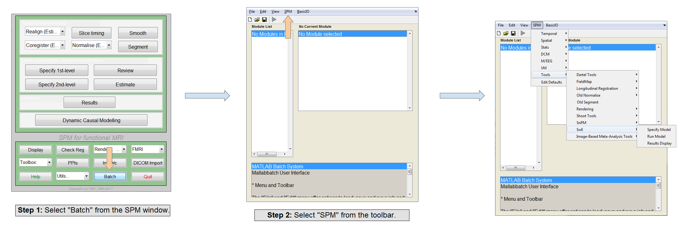
Start Matlab and run SPM.
In SPM navigate click on the "Batch" menu and select "SPM" from the Toolbar at the top of the Batch window. Under "Tools" In the drop down menu the 3 menu items for SwE should now be available.

Alternatively, to run the SwE toolbox in standalone mode, do the following:

Unzip the SwE.zip file into the SPM toolboxes folder (i.e. {path to spm}/toolbox/).
Add the folder "SwE" into your path, either using:
- For old MATLAB versions, File > Set Path > Add Folder
- For recent MATLAB versions, HOME > ENVIRONMENT > Set Path > Add Folder
- MATLAB command pathtool > Add Folder
- MATLAB command addpath …/whatever/SwE
Launch the SwE toolbox by typing swe in the command window and the following GUI should appear:

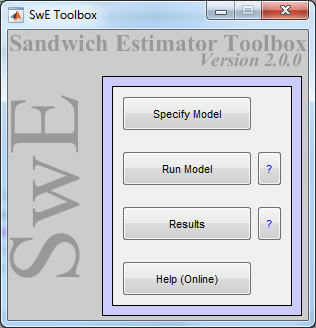
This SwE GUI has three buttons allowing to launch the three stages of an SwE analysis. Each of these stages is detailed below.

Data & design setup

To start specifying the data and design, press the button "Specify model" in the SwE GUI. This will call the SPM batch system, add the SwE tab to it and load the SwE module "Specify Model" (see image below).

SwE batch

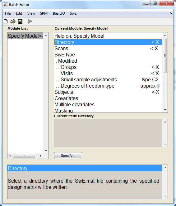
This module contains several fields that have to be filled in:

Directory:
- Select the directory where the files of the analysis will be created.
Scans:
- Select all the input images. Note that the ordering is important as other variables (Groups, Visits and Subjects) must follow the same ordering.
SwE type:
- Select between the classic or modified SwE. The classic SwE assumes that the subjects have all different covariance matrices. The modified SwE assumes that the subjects can be gathered into groups in which they share a common covariance matrix.
- If the modified version is selected, a numerical vector of group categories must be specified in the ordering of the scans. It defines in which group the subjects belong and share a common covariance matrix.
- If the modified version is selected, a numerical vector of visit (or repeated measures) categories must be specified in the ordering of the scans. For each group, the visit (or repeated measures) categories must be consistent across subjects.
- For both versions, a small samples bias adjustment must be selected. The toolbox currently offers the choice between 4 types of adjustments:
  - Type 0: The raw residuals are used to compute the SwE (no adjustments used).
  - Type 1: The raw residuals multiplied by sqrt(N/(N-p)) are used to compute the SwE, where N is the total number of input images and p is the number of covariates in the model.
  - Type 2: The adjusted residuals e_ik/sqrt(1-h_ik) are used to compute the SwE, where e_ik corresponds to the residuals of subject i at visit category k, and h_ik is the diagonal element of the hat matrix H=X’(X’X)^-1X corresponding to the residual e_ik.
  - Type 3: The adjusted residuals e_ik/(1-h_ik) are used to compute the SwE.
  Note that the simulations in Guillaume et al. (in submission) seems to favour the use of the "Type 3" adjustment.
- For both versions, a degrees of freedom estimation type must be selected. Before detailing the two options offered by the toolbox, it is important to note here that some design matrices can actually be separated into sub-design matrices such that their sets of all-zero columns are pairwise disjoints. This has an important impact on the degrees of freedom of the null distribution of the test statistics used in the SwE method and is taken into account by the toolbox for two types of estimation offered by the toolbox:
  - Naïve: The toolbox first detects the inseparable sub-design matrices involved in the contrast tested and then naïvely estimates the degrees of freedom by the number of subject present in the involved sub-design matrices minus the number of non-zero pure between covariates present in the involved sub-design matrices.
  - Approx: The estimate proposed in Guillaume et al. (in submission) is used.
Note that the simulations in Guillaume et al. (in submission) seems to show that the "Approx" option is the best option if the modified SwE is selected. Nevertheless, if the classic SwE is selected, the "Approx" option generally underestimates the degrees of freesom leading to conservative test and the option "Naïve" option may overestimate the degrees of freedom leading to liberal test. Note also that the "Approx" option requires saving a lot of images in the working directory, specifically if the classis SwE is selected, so make sure you have enough space available.

Subjects:
- Enter the vector of subjects (numerical values) in the ordering of the scans.
Covariates:
- Allow the construction of the design matrix by entering several covariates in the ordering of the scans. In this setting, the entire design matrix must be specified by adding covariates one by one.
Multiple Covariates:
- Allow the construction of the design matrix by entering a `.txt`/`.mat`file containing predefined covariates.
Masking:
- Similar to a SPM design.
Non-Parametric Wild Bootstrap:
- Select whether to do a Non-Parametric Wild Bootstrap (options are "Yes" or "No"). If "Yes" is selected, the following fields must be filled in:
Global calculation:
- Similar to a SPM design.
Global normalisation:
- Similar to a SPM design.

Once the model is specified, the SwE job can be run by pressing the green "Run Batch" button. The toolbox will then create a SwE.mat file containing all the configuration information needed for the estimation of the model parameters.

Computation of the model parameters

To start estimating the parameters of a specified model, press the button "Run model" of the SwE GUI and select the appropriate SwE.mat file. The toolbox should then compute all the estimates needed for the analysis. This may take several minutes.

Post-processing & display of results

Once the computation is done, press the "Results" button of the SwE GUI and select the appropriate SwE.mat file. For a parametric analysis, the toolbox should then open a SwE contrast manager allowing the test of several contrasts. For a wild bootstrap analysis, the toolbox will display the positive contrast which was computed.

Note that the SwE interface is very similar to the interface of a classic SPM analysis and can be used in a similar way. Nevertheless, there are some differences important to note. First, as the degrees of freedom with the SwE method may vary across voxels, for each contrast, the equivalent Z-score or 1-degree-of-freedom chi-squared image are displayed instead of the traditional t-score or F-score image (note that, for each parametric contrast, the t- or F-score image is saved in the working directory alongside the degrees of freedom image). Second, as Random Field Theory inferences have not been yet validated with the SwE method, only False Discovery Rate and uncorrected inferences are currently available in the SwE toolbox for parametric inference.

A full list of files output files, alongside a brief description of each file are given in the tables below:

Parametric Voxelwise analyses

For parametric voxelwise analyses run on input given as '.mat' files, the below files are output.

Filename	Description
`swe_vox_mask.mat`	This is the mask used during the analysis. (In previous versions of the toolbox this map was known as `mask.mat`.)
`swe_vox_beta_bb.mat`	This the the beta map for this analyis. (In previous versions of the toolbox this map was known as `beta.mat`.)
`swe_vox_cov.mat`	This is the covariance map for the beta values given in `swe_vox_beta_bb.mat`. (In previous versions of the toolbox this map was known as `cov_beta.mat`.)
`swe_vox_cov_vv.mat`	This is the covariance map for between visits. (In previous versions of the toolbox this map was known as `cov_vis.mat`.)
`swe_vox_cov_g_bb.mat`	This contains the between beta covariance maps for each group. (In previous versions of the toolbox this map was known as `cov_beta_g.mat`.)
`swe_vox_{T\|F}stat_c{c#}.mat`	This is the voxelwise parametric statistic map (T or F) for contrast `{c#}`. (In previous versions of the toolbox this map was not recorded.)
`swe_vox_{zT\|xF}stat_c{c#}.mat`	This is the voxelwise parametric equivalent statistic map (Z or 1-DF Chi-squared) for contrast `{c#}`. (In previous versions of the toolbox this map was known as `score.mat`.)
`swe_vox_{T\|F}stat_lp_c{c#}`	This is the log10 map of the voxelwise uncorrected P values for contrast `{c#}`. (In previous versions of the toolbox this map was known as `spmUncP_{#}.mat`.)
`swe_vox_edf_c{c#}.mat`	This is the error degrees of freedom map for contrast `{c#}`. (In previous versions of the toolbox this map was known as `edf_{c#}.mat`.)
`swe_vox_beta_c{c#}.mat`	This is the beta map for contrast `{c#}`. (In previous versions of the toolbox this map was known as `con_{c#}.mat`.)

For parametric analyses run on input given as '.img' or '.nii' files, the below files are output.

Filename	Description
`swe_vox_mask.nii`	This is the mask used during the analysis. (In previous versions of the toolbox this map was known as `mask.nii`.)
`swe_vox_beta_b{b#}.nii`	This the the `{b#}`th beta map for this analyis. (In previous versions of the toolbox this map was known as `beta_{b#}.nii`.)
`swe_vox_resid_y{y#}.nii`	This is the parametric residual map calculated for scan `{y#}`. (In previous versions of the toolbox this map was known as `ResI_{y#}.nii`.)
`swe_vox_cov_b{b1#}_b{b2#}.nii`	This is the covariance map between beta `{b1#}` and beta `{b2#}`. (In previous versions of the toolbox this map was known as `cov_beta_{b1#}_{b2#}.nii`.)
`swe_vox_cov_g{g#}_b{b1#}_b{b2#}.nii`	This is the covariance map for group `{#g}` between beta `{#b1}` and beta `{#b2}`. (In previous versions of the toolbox this map was known as `cov_beta_g_{g#}_{b1#}_{b2#}.nii`.)
`swe_vox_cov_g{g#}_v{v1#}_v{v2#}.nii`	This is the covariance map for group `{#g}` between visit `{#v1}` and visit `{#v2}`. (In previous versions of the toolbox this map was known as `cov_vis_{g#}_{v1#}_{v2#}.nii`.)
`swe_vox_edf_c{c#}.nii`	This is the error degrees of freedom map for contrast `{c#}`. (In previous versions of the toolbox this map was known as `edf_{c#}.nii`.)
`swe_vox_{T\|F}stat_lp_c{c#}.nii`	This is the log10 map of the voxelwise uncorrected P values for contrast `{c#}`. (In previous versions of the toolbox this map was known as `spmUncP_{c#}.nii`.)
`swe_vox_{T\|F}stat_c{c#}.nii`	This is the voxelwise parametric statistic map (T or F) for contrast `{c#}`. (In previous versions of the toolbox this map was known as `spm?_{c#}.nii`.)
`swe_vox_{zT\|xF}stat_c{c#}.nii`	This is the voxelwise parametric equivalent statistic map (Z or 1-DF Chi-Squared) for contrast `{c#}`. (In previous versions of the toolbox this map was known as `score.nii`.)
`swe_vox_beta_c{c#}.nii`	This is the beta map for contrast `{c#}`. (In previous versions of the toolbox this map was known as `con_{c#}.nii`.)

Non-Parametric Clusterwise analyses

For non-parametric clusterwise analyses run on input given as '.mat' files, the below files are output.

Filename	Description
`swe_vox_mask.mat`	This is the mask used during the analysis. (In previous versions of the toolbox this map was known as `mask.mat`.)
`swe_vox_beta_bb.mat`	This is the beta map. (In previous versions of the toolbox this map was known as `beta.mat`.)
`swe_vox_{T\|F}stat_c{c#}.mat`	This is the voxelwise parametric statistic map (T or F) for contrast `{c#}`. (In previous versions of the toolbox this map was not recorded.)
`swe_vox_{zT\|xF}stat_c{c#}.mat`	This is the voxelwise parametric equivalent statistic map (Z or 1-DF Chi-Squared) for contrast `{c#}`. (In previous versions of the toolbox this map was known as `score.mat` for `{c#}=001`.)
`swe_vox_{zT\|xF}stat-WB_c{c#}.mat`	This is the voxelwise non-parametric equivalent statistic map (Z or 1-DF Chi-Squared) for contrast `{c#}`, derived from the non-parametric uncorrected P values in `swe_vox_{T\|F}stat_lp-WB_c{c#}.mat`. (In previous versions of the toolbox this map was not recorded.)
`swe_vox_{T\|F}stat_lp-WB_c{c#}.mat`	This is the log10 map of the voxelwise uncorrected P values for contrast `{c#}`. (In previous versions of the toolbox this map was known as `luncP_{pn}.mat`*.)
`swe_vox_{T\|F}stat_lpFWE-WB_c{c#}.mat`	This is the log10 map of the voxelwise bootstrap-calculated FWE P values for contrast `{c#}`. (In previous versions of the toolbox this map was known as `lfwerP_{pn}.mat`*.)
`swe_vox_{T\|F}stat_lpFDR-WB_c{c#}.mat`	This is the log10 map of the voxelwise bootstrap-calculated FDR P values for contrast `{c#}`. (In previous versions of the toolbox this map was known as `lfdrP_{pn}.mat`*.)
`swe_clustere_{T\|F}stat_lpFWE-WB_c{c#}.mat`	This is the log10 map of the clusterwise bootstrap-calculated FWE P values for contrast `{c#}`. (In previous versions of the toolbox this map was known as `lclusterFwerP_{pn}_perElement.mat`.)
`swe_vox_resid_y{y#}.mat`✝	These are the wild-bootstrap generated residuals obtained for scan `{y#}`. (In previous versions of the toolbox this map was known as `ResWB_{y#}.mat`.)
`swe_vox_fit_y{y#}.mat`✝	These are the fitted values obtained for scan `{y#}` calculated using the wild-bootstrap generated residuals given in `swe_vox_resid_y{y#}.mat`. (In previous versions of the toolbox this map was known as `YfittedWB_{y#}.mat`.)

For non-parametric clusterwise analyses run on input given as '.img' or '.nii' files, the below files are output.

Filename	Description
`swe_vox_mask.nii`	This is the mask used during the analysis. (In previous versions of the toolbox this map was known as `mask.nii`.)
`swe_vox_{T\|F}stat_c{c#}.nii`	This is the voxelwise parametric statistic map (T or F) for contrast `{c#}`. (In previous versions of the toolbox this map was not recorded.)
`swe_vox_{zT\|xF}stat_c{c#}.nii`	This is the voxelwise parametric equivalent statistic map (Z or 1-DF Chi-Squared) for contrast `{c#}`. (In previous versions of the toolbox this map was known as `score.nii` for `{c#}=001`.)
`swe_vox_{zT\|xF}stat-WB_c{c#}.nii`	This is the voxelwise non-parametric equivalent statistic map (Z or 1-DF Chi-Squared) for contrast `{c#}`, derived from the non-parametric uncorrected P values in `swe_vox_{T\|F}stat_lp-WB_c{c#}.nii`. (In previous versions of the toolbox this map was not recorded.)
`swe_vox_{T\|F}stat_lp-WB_c{c#}.nii`	This is the log10 map of the voxelwise uncorrected P values for contrast `{c#}`. (In previous versions of the toolbox this map was known as `lP{+-}.nii`*.)
`swe_vox_{T\|F}stat_lpFWE-WB_c{c#}.nii`	This is the log10 map of the voxelwise bootstrap-calculated FWE P values for contrast `{c#}`. (In previous versions of the toolbox this map was known as `lP_FWE{+-}.nii`*.)
`swe_vox_{T\|F}stat_lpFDR-WB_c{c#}.nii`	This is the log10 map of the voxelwise bootstrap-calculated FDR P values for contrast `{c#}`. (In previous versions of the toolbox this map was known as `lP_FDR{+-}.nii`*.)
`swe_clustere_{T\|F}stat_lpFWE-WB_c{c#}.nii`	This is the log10 map of the clusterwise bootstrap-calculated FWE P values for contrast `{c#}`. (In previous versions of the toolbox this map was known as `lP_clusterFWE{+-}.nii`*.)
`swe_vox_resid_y{y#}.nii`✝	These are the wild-bootstrap generated residuals obtained for scan `{y#}`. (In previous versions of the toolbox this map was known as `ResWB_{y#}.nii`.)
`swe_vox_fit_y{y#}.nii`✝	These are the fitted values obtained for scan `{y#}` calculated using the wild-bootstrap generated residuals given in `swe_vox_resid_y{y#}.nii`. (In previous versions of the toolbox this map was known as `YfittedWB_{y#}.nii`.)

Non-Parametric TFCE analyses

For non-parametric TFCE analyses run on input given as '.img' or '.nii' files, the below files are output.

Filename	Description
`swe_vox_mask.nii`	This is the mask used during the analysis. (In previous versions of the toolbox this map was known as `mask.nii`.)
`swe_vox_{T\|F}stat_c{c#}.nii`	This is the voxelwise parametric statistic map (T or F) for contrast `{c#}`. (In previous versions of the toolbox this map was not recorded.)
`swe_vox_{zT\|xF}stat_c{c#}.nii`	This is the voxelwise parametric equivalent statistic map (Z or 1-DF Chi-Squared) for contrast `{c#}`. (In previous versions of the toolbox this map was known as `score.nii` for `{c#}=001`.)
`swe_vox_{zT\|xF}stat-WB_c{c#}.nii`	This is the voxelwise non-parametric equivalent statistic map (Z or 1-DF Chi-Squared) for contrast `{c#}`, derived from the non-parametric uncorrected P values in `swe_vox_{T\|F}stat_lp-WB_c{c#}.nii`. (In previous versions of the toolbox this map was not recorded.)
`swe_vox_{T\|F}stat_lp-WB_c{c#}.nii`	This is the log10 map of the voxelwise uncorrected P values for contrast `{c#}`. (In previous versions of the toolbox this map was known as `lP{+-}.nii`*.)
`swe_vox_{T\|F}stat_lpFWE-WB_c{c#}.nii`	This is the log10 map of the voxelwise bootstrap-calculated FWE P values for contrast `{c#}`. (In previous versions of the toolbox this map was known as `lP_FWE{+-}.nii`*.)
`swe_vox_{T\|F}stat_lpFDR-WB_c{c#}.nii`	This is the log10 map of the voxelwise bootstrap-calculated FDR P values for contrast `{c#}`. (In previous versions of the toolbox this map was known as `lP_FDR{+-}.nii`*.)
`swe_tfce_c{c#}.nii`	This is the parametric TFCE statistic for contrast `{c#}`.
`swe_tfce_lp-WB_c{c#}.nii`	This is the log10 map of the TFCE bootstrap-calculated uncorrected P values for contrast `{c#}`.
`swe_tfce_lpFWE-WB_c{c#}.nii`	This is the log10 map of the TFCE bootstrap-calculated FWE P values for contrast `{c#}`.
`swe_vox_resid_y{y#}.nii`✝	These are the wild-bootstrap generated residuals obtained for scan `{y#}`. (In previous versions of the toolbox this map was known as `ResWB_{y#}.nii`.)
`swe_vox_fit_y{y#}.nii`✝	These are the fitted values obtained for scan `{y#}` calculated using the wild-bootstrap generated residuals given in `swe_vox_resid_y{y#}.nii`. (In previous versions of the toolbox this map was known as `YfittedWB_{y#}.nii`.)

*Note: For non-parametric analyses {c#} is 001 for activation and 002 for deactivation. In previous versions of the toolbox these were represented with either a +/- or p/n.

✝ These maps will be removed once an analysis has been run. They will only be retained if an analysis is ended prematurely.