SwE: Example Sandwich Estimator Toolbox for Longitudinal & Repeated Measures Data A toolbox for SPM By Bryan Guillaume & Thomas Nichols

 

---

This page... News Introduction Manual FMRI worked example Download References Contact

Worked Example In this section, we analyze with the SwE toolbox a reapeated-measures fMRI dataset from Henson, R.N.A, Shallice, T., Gorno-Tempini, M.-L. & Dolan, R.J (2002). Face repetition effects in implicit and explicit memory tests as measured by fMRI. Cerebral Cortex, 12, 178-186. The same dataset has also been analyzed by SPM in Section 30.4 of the SPM12 manual (the manual and the dataset can be found here). More precisely, the dataset consists of 36 contrast images obtained after using an "informed" basis set (consisting of the canonical HRF and its two partial derivatives with respect to time and dispersion) in single-subject fMRI analyses applied on 12 subject fMRI scans.

---

The analysis with the SwE toolbox

Here, we assume that the SwE toolbox has already been downloaded and installed correctly (see the manual if it is not the case).

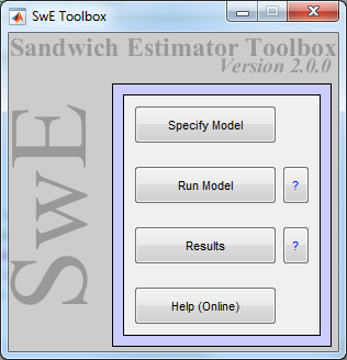
To start the toolbox, type swe in the MATLAB command window and the following GUI should appear:

Press the "Specify model" button of the SwE GUI and the following batch system with the SwE module "Specify Model" already loaded should appear:

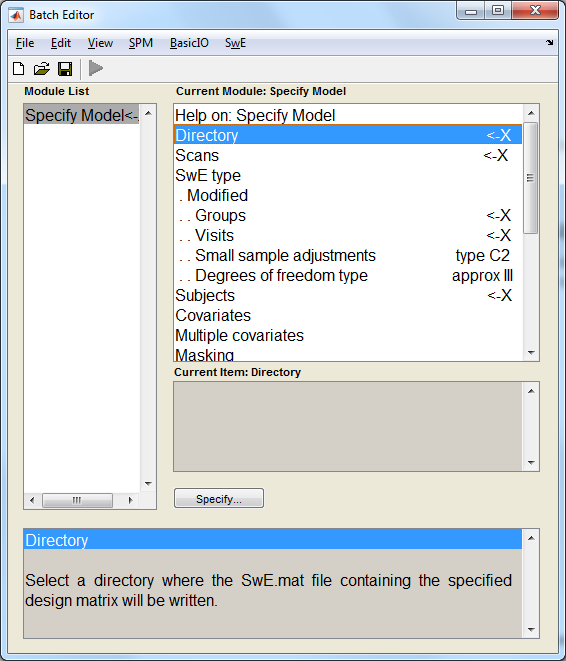
Highlight the field "Directory", press the button "Specify" and select the directory where the files of the analysis will be created.

Highlight the field "Scans", press the button "Specify" and select in numerical order the 36 contrasts images (con_0003.img, con_0004.img,..., con_0038.img) that can be found in the folder "cons_informed" of the downloaded file "face_rfx.zip". Note that the ordering of the scans is important as other variables (Groups, Visits and Subjects) must follow the same ordering. The correspondance of each of these scans is shown in the following table:

	Canonical HRF	Temporal derivative	Dispersion derivative
Subject 1	con_0003.img	con_0015.img	con_0027.img
Subject 2	con_0004.img	con_0016.img	con_0028.img
…	…	…	…
Subject 12	con_0014.img	con_0026.img	con_0038.img

For our example, we may assume that all the subjects share a common covariance matrix. Therefore, highlight the field "SwE type" and select "*Modified" from the "Current Item: SwE type" box. Then, highlight the field "Groups" item under "SwE type", press the "Specify" button and enter a column vector containing 36 ones by, for example, using the MATLAB command ones(36,1).

Highlight the field "Visits", press the "Specify" button and enter a vector of visit/repeated-measure categories. For our example, there are three repeated-measures categories corresponding to 1) the canonical HRF, 2) the temporal derivative and 3) the dispersion derivative. This can be specified by using the MATLAB command kron((1:3),ones(1,12)), which will generate a column vector containing 12 ones, 12 twos, and 12 threes.

Highlight the field "Small sample adjustments" and select the type of bias corrective factor to be applied to the residuals prior their use in the estimation of the SwE. Based on extensive simulations in Guillaume et al. (2014) [PDF] and Guillaume (2015) [PDF], we recommend leaving the Small sample adjustments to the default value, "type C2".

Highlight the field "Degrees of freedom type" to select the type of estimation used for degrees of freedom. Again, based on extensive simulations, we suggest using the default value, "approx III". (The "approx II" Degrees of freedom type may be better than "approx III" but is only safe if using a balanced design).

Highlight the field "Subjects", press the "Specify" button and specify the vector of subjects. In our example, this can be done by again using the MATLAB command kron(ones(1,3),1:12), which generates a column vector containin 1, 2, 3, . . ,12 three times

Next you need to specify the three covariates. To create a covariate, first click the "Covariates" field, then click "New: Covariate" in the lower box. That will add a section above for the new covariate. Click on the "Name" field, then on the "Specify" button, and enter the covariate name. The first covariate is "Canonical HRF". Next, you click the "Vector" field, then the "Specify" button to enter the vector for the covariate, which for the canonical HRF function is kron([1 0 0],ones(1,12)).

There are three covariates, so you need to repeat the process for the covariate for the temporal derivative and for the dispersion derivative.

Highlight the field "Covariates" again, press "New: Covariate"; click the "Name" field and enter the name of the second covariate, "Temporal derivative". Click the "Vector" field, and enter the vector, which for the temporal derivative is, kron([0 1 0],ones(1,12)).

Highlight the field "Covariates" one last time, press "New: Covariate"; click the "Name" field and enter the name of the second covariate, "Dispersion derivative". Click the "Vector" field, and enter the vector, which for the temporal derivative is, kron([0 0 1],ones(1,12)).

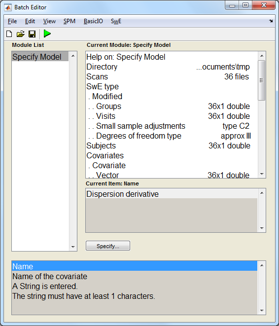
The remaining fields are similar to a classic SPM batch job and can be left unchanged for our example. The batch window should then look like this:

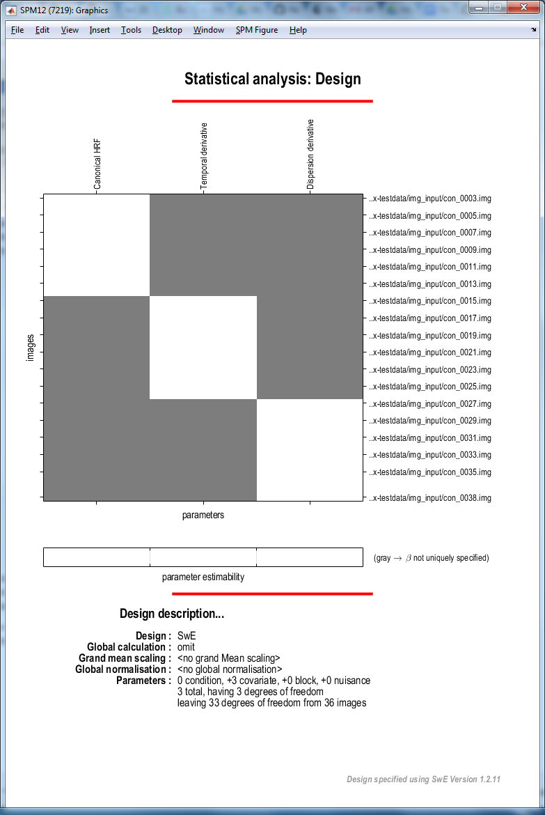
Finally, push the green "Run Batch" button. An SwE.mat file containing all the information related to the data and design should then be created in the specified working directory and the following window showing the design matrix should appear:

To start estimating the parameters of this specified model, press the button "Run model" of the SwE GUI and select the SwE.mat file just created. The toolbox should then compute all the estimates needed for the analysis and update the SwE.mat file.

Once the computation is done, press the "Results" button of the SwE GUI and select the updated SwE.mat file. The toolbox should then open the following SwE contrast manager allowing the test of several contrasts:

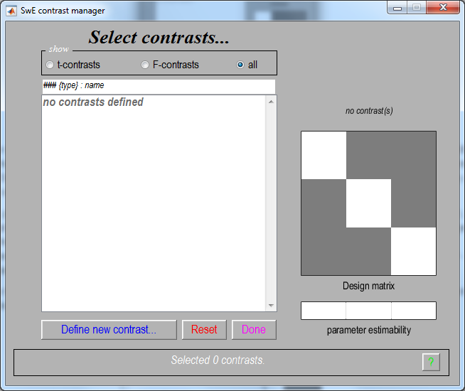
In the contrast manager, press "Define new contrast", select F-contrast in the "type" section, enter the MATLAB command eye(3) in the "contrast" section, enter "Faces vs Baseline: Informed" in the "name" section and press the "OK" button. This contrast will reveal voxels that exhibit some form of event-related responses captured by at least one of the three basis functions.

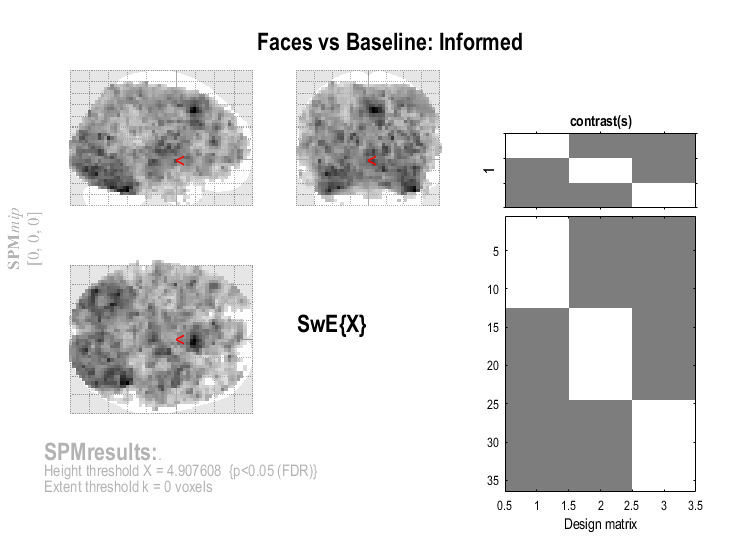
Now, press the "Done" button in the SwE contrast manager, press the "none" button (section "apply masking"), accept "Faces vs Baseline: Informed" as title for comparison and the toolbox will compute the inferences images (i.e. the F-score image swe_vox_Fstat_c01.nii, the equivalent chi-squared-score image swe_vox_xFstat_c01.nii and the degrees of freedom image swe_vox_edf_c01.nii) in the working directory. Note that it can take several minutes for F-contrasts with a rank superior to 1, like it is the case here.

Once the computation is done, press the "FDR" button, validate "0.05" as a FDR p-value, validate "0" as extent threshold and the toolbox should display the following result:

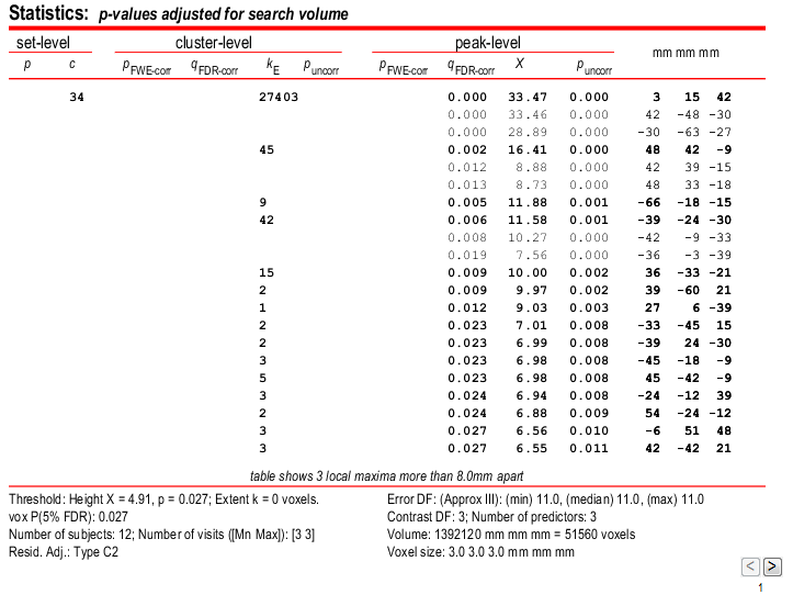
Note that, like this, it is difficult to visualise where the effects are exactly. Therefore, in order to see better which areas of the brain are activated, you can press the "whole brain" button and a list summarising the most important activations in the brain should appear:

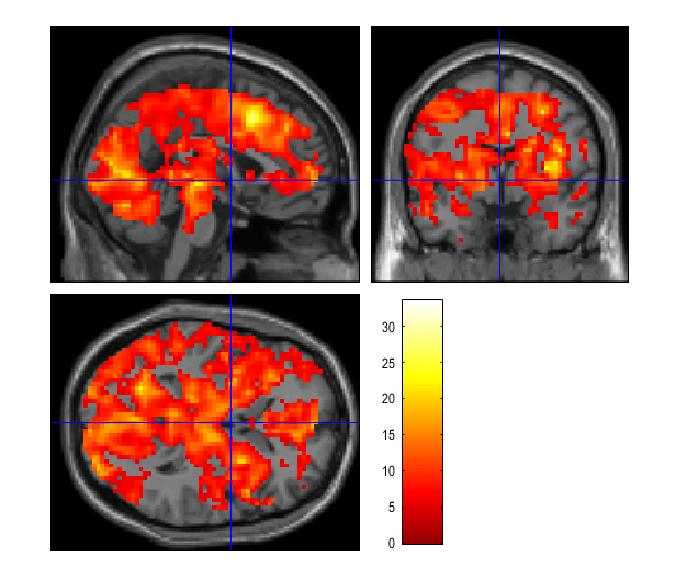
You can also select "sections" in the "overlay" menu and select the image single_subj_T1.nii situated in the subfolder "canonical" of your SPM12 main folder. You should then get the following display:

You can navigate through it in order to see more pricesely the areas of activation. Note that you may also want to impose a more restrective threshold. To do so, go into "Contrasts" > "Significance level" > "Change..." as shown below:

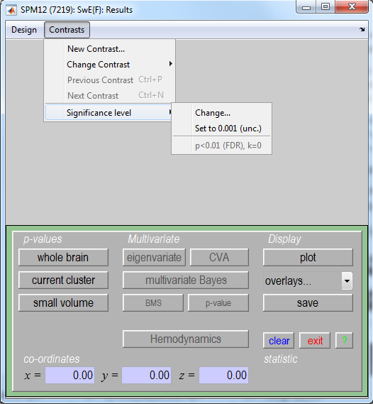
Then, you can reselect an FDR correction (button "FDR"), change the significance level (e.g., 0.01) and eventually the extent threshold (e.g., 10 voxels) or select an uncorrected threshold instead (button "none").

Similarly to the SPM analysis in Section 30.4 of the SPM manual, you can test contrasts only focused on one basis function. To do so, go into "Contrasts" > "New Contrast..." and you will go back to the SwE contrast manager. There, you can specify the following contrasts:

• t-contrast [1 0 0] (i.e. positive effects on the canonical HRF)
• F-contrast [0 1 0] (i.e. positive or negative effects on the temporal derivative)
• F-contrast [0 0 1] (i.e. positive or negative effects on the dispersion derivative)

and restart the procedure to compute the inference images and display the results for each new contrast.

Testing the three new contrasts and using a FDR correction at 0.05 level of significance, you should get the three following displays:

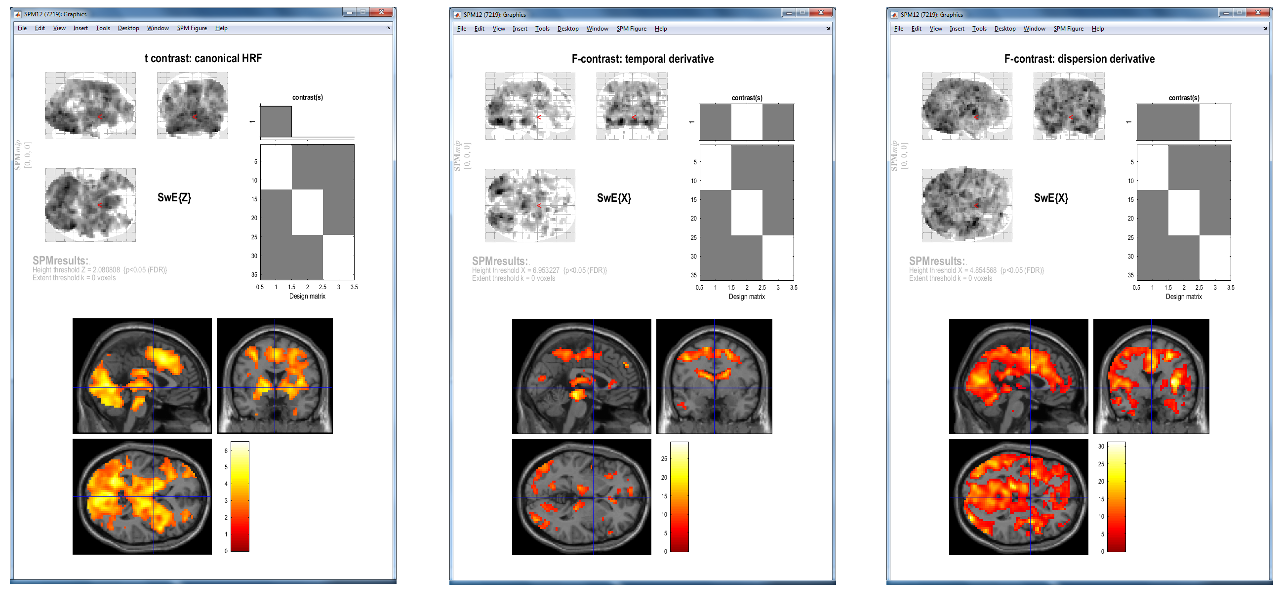
Note here that, overall, the areas of activation obtained with the SwE method are similar to those obtained with the SPM procedure (see Section 30.4 of the manual). Nevertheless, if we look more in details, we can observe differences between the two methods. This is mainly due to these three facts:

1. Here, FDR corrections are used while it was Random Field Theory corrections with the SPM procedure. Note that the FDR correction can be enabled in a classic SPM analysis by setting the SPM global variable defaults.stats.topoFDR to 0 instead of 1. Note also that, in order to make a more objective comparison, one can use an uncorrected threshold (with the same significance level) for both methods and compare the results.
2. The SPM procedure assumes and estimates a unique covariance structure for all the voxels in the brain. This can lead to invalid inferences in voxels where the true covariance structure is different from the one estimated. In contrast, the SwE estimates a different covariance matrix for each voxel, making the inferences valid for each voxel.
3. Due to the fact that the SwE procedure estimates a covariance matrix for each voxel in the brain, more degrees of freedom have to be used compared to the SPM procedure which estimates only one unique covariance structure for the whole brain. This makes the SwE procedure less powerful than the SPM procedure.