|
|
SnPM13 ManualA fMRI Example |
fMRI Group Analysis Example
In this section, we analyze multi-subject event-related fMRI data with the SnPM13 software. The data-set used in this example is available on the SPM website: Multi-subject event-related fMRI - Repetition priming
The reference is: Henson, R.N.A, Shallice, T., Gorno-Tempini, M.-L. & Dolan, R.J (2002). Face repetition effects in implicit and explicit memory tests as measured by fMRI. Cerebral Cortex, 12, 178-186.
This data have also been analyzed by SPM. The details can be found at SPM website.
We will give two standard methods to analyze the data by using nonparametric methods:
The Example Data
The data are from a study on face repetition effects in implicit and explicit memory tests (Henson et al. 2002; see above).
In this study, twelve volunteers (six male; aged 22-42 years, median 29 years) participated in the experiment. Faces of famous and nonfamous people were presented to the subjects for 500 ms, and replaced by a baseline of an oval chequerboard throughout the interstimulus interval. Each subject was scanned during the experiment and his or her fMRI images were obtained.
Each subject's data were analyzed, creating a difference image between faces and chequerboad (baseline) watchings. So each image here is the contrast image for each subject.
Under the null hypothesis we can permute the labels of the effects of interest. One way of implimenting this with contrast images is to randomly change the sign of each subject's contrast. This sign-flipping approach can be justified by a symmetric distribution for each voxel's data under the null hypothesis. While symmetry may sound like a strong assumption, it is weaker than Normality, and can be justified by a subtraction of two sample means with the same (arbitrary) distribution.
Hence the null hypothesis here is:
H0: The symmetric distribution of (the voxel values of the) subjects' contrast images have zero mean.
Exchangeability of Second Level fMRI Data
fMRI data presents a special challenge for nonparametric methods. Because fMRI data exhibits temporal autocorrelation, an assumption of exchangeability of scans within subject is not tenable. However, to analyze a group of subjects for population inference, we need to only assume exchangeability of subjects. The conventional assumption of independent subjects implies exchangeability, and hence a single exchangeability block (EB) consisting of all subjects.
(On a technical note, the assumption of exchangeability can actually be relaxed for the one-sample case considered here. A sufficient assumption for the contrast data to have a symmetric distribution, is for each subject's contrast data to have a symmetric but possibly different distribution. Such differences between subjects violates exchangeability of all the data; however, since the null distribution of the statistic of interest is invariant with respect to sign-flipping, the test is valid.)
Nonparametric Group Analysis
(Without smoothed variance t)
In matlab (in a new directory !) type
-
spm fmri
SPM is launched and the GUI is displayed. Click on the Batch button to open the SPM batch window.
Design your experiment
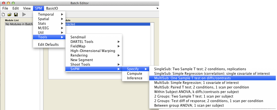
In the SPM menu, under Tools -> SnPM -> Specify, select MultiSub: One Sample T test on diffs/contrasts
Then fill in the required fields as follows:
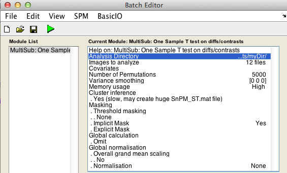
Analysis directory: Select the directory in which the analysis files will be stored.Images to analyze: Select all scan files from thecons_candirectory (i.e.con_0006.img->con_0017.img).
Cluster inference:Yes (slow, may create huge SnPM_ST.mat file).
CovariatesNumber of permutationsVariance smoothingMemory usageMaskingGlobal calculationGlobal normalisation
Finally, the Batch window is as below:
The start button in SPM batch window is now green  , click on it to run the job.
SnPM will now create the file SnPMcfg.mat. and show the Design Matrix in the Graphics window.
Compute your experiment
In the SPM menu, under Tools -> SnPM, select Compute.
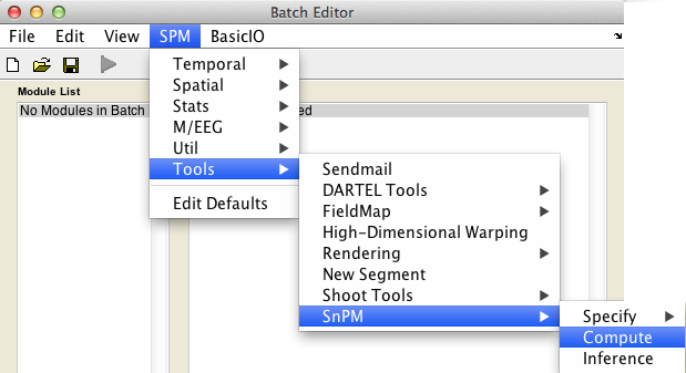
Then fill in the required field as follows:
SnPMcfg.mat configuration file: Select theSnPMcfg.matfile just created.
The start button in SPM batch window is now green  , click on it to run the job.
The computation should take between 5 and 10 minutes depending on your computer.In one of the SnPM window, it will show the percentage of the completeness, and in the matlab window, the permutation step that is being performed will be listed.
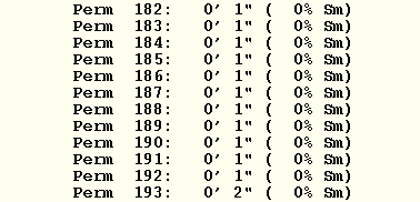
Note that it shows how many minutes and seconds spent on each permutation. The number in parentheses is the percentage of time spent on variance smoothing. Since we choose no variance smoothing, this is 0%.
Inference
In the SPM menu, under Tools -> SnPM, select Inference.
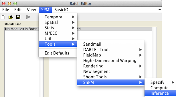
Cluster-wise inference
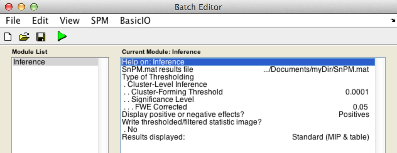
For cluster-wise inference with p < 0.05 FWE corrected using a cluster-forming threshold of p < 0.0001, fill in the required field as follows:
SnPM.mat results file: Select theSnPM.matfile just created.Type of thresholding: Selectcluster-wise inferenceCluster-forming threshold: Type0.0001
Display positive or negative effects?Results displayed
Finally, the Batch window is as below:
The start button in SPM batch window is now green  , click on it to run the job.
SnPM will then plot a MIP of those voxels surviving the SnPM critical threshold.

Voxel-wise inference
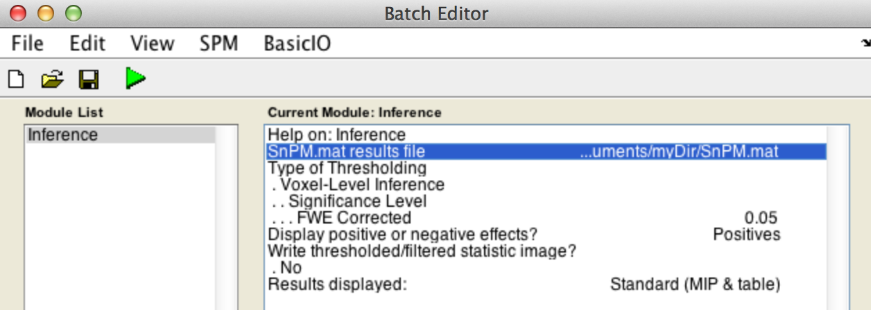
For voxel-wise inference with p < 0.05 FWE corrected, fill in the required field as follows:
SnPM.mat results file: Select theSnPM.matfile just created.
Type of thresholdingDisplay positive or negative effects?Results displayed
Finally, the Batch window is as below:
The start button in SPM batch window is now green  , click on it to run the job.
SnPM will then plot a MIP of those voxels surviving the SnPM critical threshold (this value is displayed at the bottom of the image and for this data set should be 7.92).

You can then use this value in SPM (in the RESULTS section, say 'No' to corrected height threshold, and then type in 7.9248 for the threshold) and take advantage of SPMs rendering routines (not available in SnPM).
Note that the SnPM threshold is lower than the SPM threshold (9.07). Consequently, SnPM shows more active voxels.
Nonparametric Analysis
(With smoothed variance t, Pseudo-t)
Note that the result just obtained looks "jaggedy". That is, while the image data is smooth (check the con* images), the t statistic image is rough. A t statistic is a estimate divided by a square root of the variance of the estimate, and this roughness is due to uncertainty of the variance estimate; this uncertainty is especially bad when the degrees of freedom are low (here, 11). By smoothing the variance before creating a t ratio we can eliminate this roughness and effectively increase our degrees of freedom, increasing our power.
Create a new directory for the smoothed variance results. In matlab type
-
spm fmri
SPM is launched and the GUI is displayed. Click on the Batch button to open the SPM batch window.
Design your experiment
In the SPM menu, under Tools -> SnPM -> Specify, select MultiSub: One Sample T test on diffs/contrasts

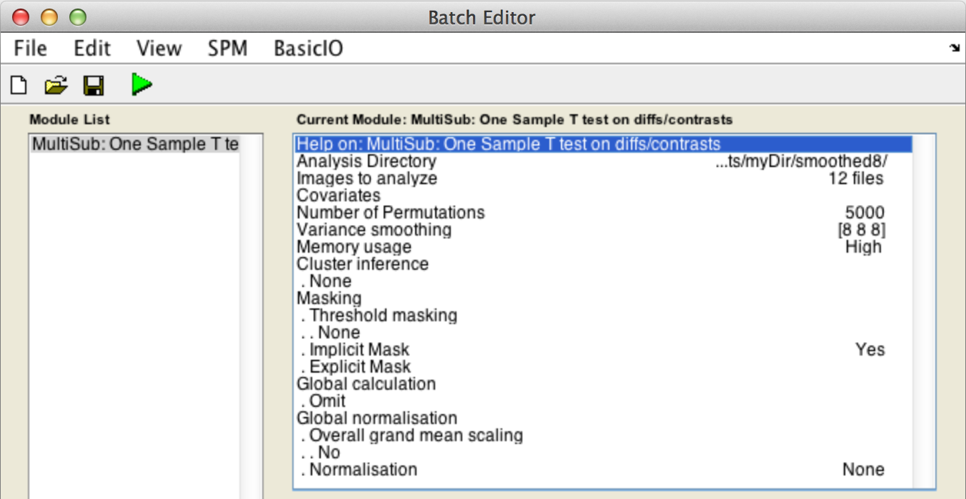
Then fill in the required fields as follows:
Analysis directory: Select the directory in which the analysis files will be stored.Images to analyze: Select all scan files from thecons_candirectory (i.e.con_0006.img->con_0017.img).
Variance smoothing:8 8 8.
CovariatesNumber of permutationsMemory usageMaskingGlobal calculationGlobal normalisation
Finally, the Batch window is as below:
The start button in SPM batch window is now green  , click on it to run the job.
SnPM will now create the file SnPMcfg.mat and show the Design Matrix in the Graphics window.
Compute your experiment
In the SPM menu, under Tools -> SnPM, select Compute.

Then fill in the required field as follows:
SnPMcfg.mat configuration file: Select theSnPMcfg.matfile just created.
The start button in SPM batch window is now green  , click on it to run the job.
In the matlab window, the permutation step that is being performed will be listed.
Voxel-wise inference
For voxel-wise inference with p < 0.05 FWE corrected, fill in the required field as follows:
SnPM.mat results file: Select theSnPM.matfile just created.
Type of thresholdingDisplay positive or negative effects?Results displayed
Finally, the Batch window is as below:

The start button in SPM batch window is now green  , click on it to run the job.
SnPM will then plot a MIP of those voxels surviving the SnPM critical threshold (this value is displayed at the bottom of the image and for this data set should be 5.09). Observe how there are both more suprathreshold voxels, and that the image is smoother.

Very important!!! This is not a t image. So you cannot apply this threshold to a t image in SPM. You can, however, create overlay images with the following:
- Use 'Display' to select the image you would like for a background. Via the keyboard only you could do...
				Img =  spm_select(1,'image','select background reference');

spm_image('init',Img) - Overlay the filtered image
spm_orthviews('addimage',1,'SnPM_filtered.nii')


