|
|
SnPM13 ManualA PET Example |
PET Single-Subject Example
In this section we analyze a simple motor activation experiment with the SnPM software. The aim of this example is three-fold:- Demonstrate the steps of an SnPM analysis
- Explain and illustrate the key role of exchangeability
- Provide a bench mark analysis for validation of an SnPM installation
The Example Data
This example will use data from a simple primary motor activation experiment. The motor stimulus was the simple finger opposition task. For the activation state subjects were instructed to touch their thumb to their index finger, then to their middle finger, to their ring finger, to their pinky, then repeat; they were to do this at a rate of 2 Hz, as guided by a visual cue. For baseline, there was no finger movement, but the visual cue was still present. There was no randomization and the task labeling used was
- A B A B A B A B A B A B
You can download the data from SPM website. We are indebted to Paul Kinahan and Doug Noll for sharing this data. See this reference for details: Noll D, Kinahan et al. (1996) "Comparison of activation response using functional PET and MRI" NeuroImage 3(3):S34.
Currently this data is normalized with SPM94/95 templates, so the activation site will not map correctly to ICBM reference images.
Before you touch the computer
The most important consideration when starting an analysis is the choice of exchangeability block size and the impact of that choice on the number of possible permutations. We don't assume that the reader is familiar with either exchangeability or permutation tests, so we'll attempt to motivate the permutation test through exchangeability, then address these central considerations.
Exchangeability
First we need some definitions.
- Labels & Labelings A designed experiment entails repeatedly collecting data under conditions that are as similar as possible except for changes in an experimental variable. We use the term labels to refer to individual values of the experimental variable, and labeling to refer to a particular assignment of these values to the data. In a randomized experiment the labeling used in the experiment comes from a random permutation of the labels; in a non-randomized experiment the labeling is manually chosen by the experimenter.
- Null Hypothesis The bulk of statistical inference is built upon what happens when the experimental variable has no effect. The formal statement of the "no effect" condition is the null hypothesis.
- Statistic We will need to use the term statistic in it's most general sense: A statistic is a function of observed data and a labeling, usually serving to summarize or describe some attribute of the data. Sample mean difference (for discrete labels) and the sample correlation (for continuous labels) are two examples of statistics.
We can now make a concise statement of exchangeability. Observations are said to be exchangeable if their labels can be permuted with out changing the expected value of any statistic. We will always consider the exchangeability of observations under the null hypothesis.
We'll make this concrete by defining these terms with our data, considering just one voxel (i.e 12 values). Our labels are 6 A's and 6 B's. A reasonable null hypothesis is "The A observations have the same distribution as the B observations". For a simple statistic we'll use the difference between the sample means of the A & B observations. If we say that all 12 scans are exchangeable under the null hypothesis we are asserting that for any permutation of A's and B's applied to the data the expected value of the difference between A's & B's would be zero.
This should seem reasonable: If there is no experimental effect the labels A and B are arbitrary, and we should be able to shuffle them with out changing the expected outcome of a statistic.
But now consider a confound. The most ubiquitous confound is time. Our example data took over two hours to collect, hence it is reasonable to suspect that the subject's mental state changed over that time. In particular we would have reason to think that difference between the sample means of the A's and B's for the labeling
- A A A A A A B B B B B B
would not be zero under the null because this labeling will be sensitive to early versus late effects. We have just argued, then, that in the presence of temporal confound all 12 scans are not exchangeable.
Exchangeability Blocks
The permutation approach requires exchangeability under the null hypothesis. If all scans are not exchangeable we are not defeated, rather we can define exchangeability blocks (EBs), groups of scans which can be regarded as exchangeable, then only permute within EB.
We've made a case for the non-exchangeability of all 12 scans, but what if we considered groups of 4 scans. While the temporal confound may not be eliminated its magnitude within the 4 scans will be smaller simply because less time elapses during those 4 scans. Hence if we only permute labels within blocks of 4 scans we can protect ourselves from temporal confounds. In fact, the most temporally confounded labeling possible with an EB size of 4 is
- A A B B A A B B A A B B
Number of Permutations
This brings us to the impact of EB size on the number of permutations. The table below shows how EB size affects the number of permutations for our 12 scan, 2 condition activation study. As the EB size gets smaller we have few possible permutations.
| EB size | Num EB's | Num Permutations | ||
| 12 | 1 | 12C6 | = | 924 |
| 6 | 2 | (6C3)2 | = | 400 |
| 4 | 3 | (4C2)3 | = | 216 |
| 2 | 6 | (2C1)6 | = | 64 |
This is important because the crux of the permutation approach is calculating a statistic for lots of labelings, creating a permutation distribution. The permutation distribution is used to calculate significance: the p-value of the experiment is the proportion of permutations with statistic values greater than or equal to that of the correct labeling. But if there are only, say, 20 possible relabelings and the most significant result possible will be 1/20=0.05 (which would occurs if the correctly labeled data yielded the largest statistic).
Hence we have to make a trade off. We want small EBs to ensure exchangeability within block, but very small EBs yield insufficient numbers of permutations to describe the permutation distribution well, and hence assign significance finely. We usually will use the smallest EB that allows for at least hundreds of permutations (unless, of course, we were untroubled by temporal effects).
Start SnPM13
It is intended that you are actually sitting at a computer and are going through these steps with Matlab. We assume that you either have the sample data on hand or a similar, single subject 2 condition with replications data set.
First, if you have a choice, choose a machine with lots of memory. We found that this example causes the Matlab process to grow to at least 90MB.
Create a new directory where the results from this analysis will go. Either start Matlab in this directory, or cd to this directory in an existing Matlab session.
In Matlab, start SnPM by typing
-
spm fmri
SPM is launched and the GUI is displayed. Click on the Batch button to open the SPM batch window.
Design your experiment
In the SPM menu, under Tools -> SnPM -> Specify, select SingleSub: Two Sample T test; 2 conditions, replications
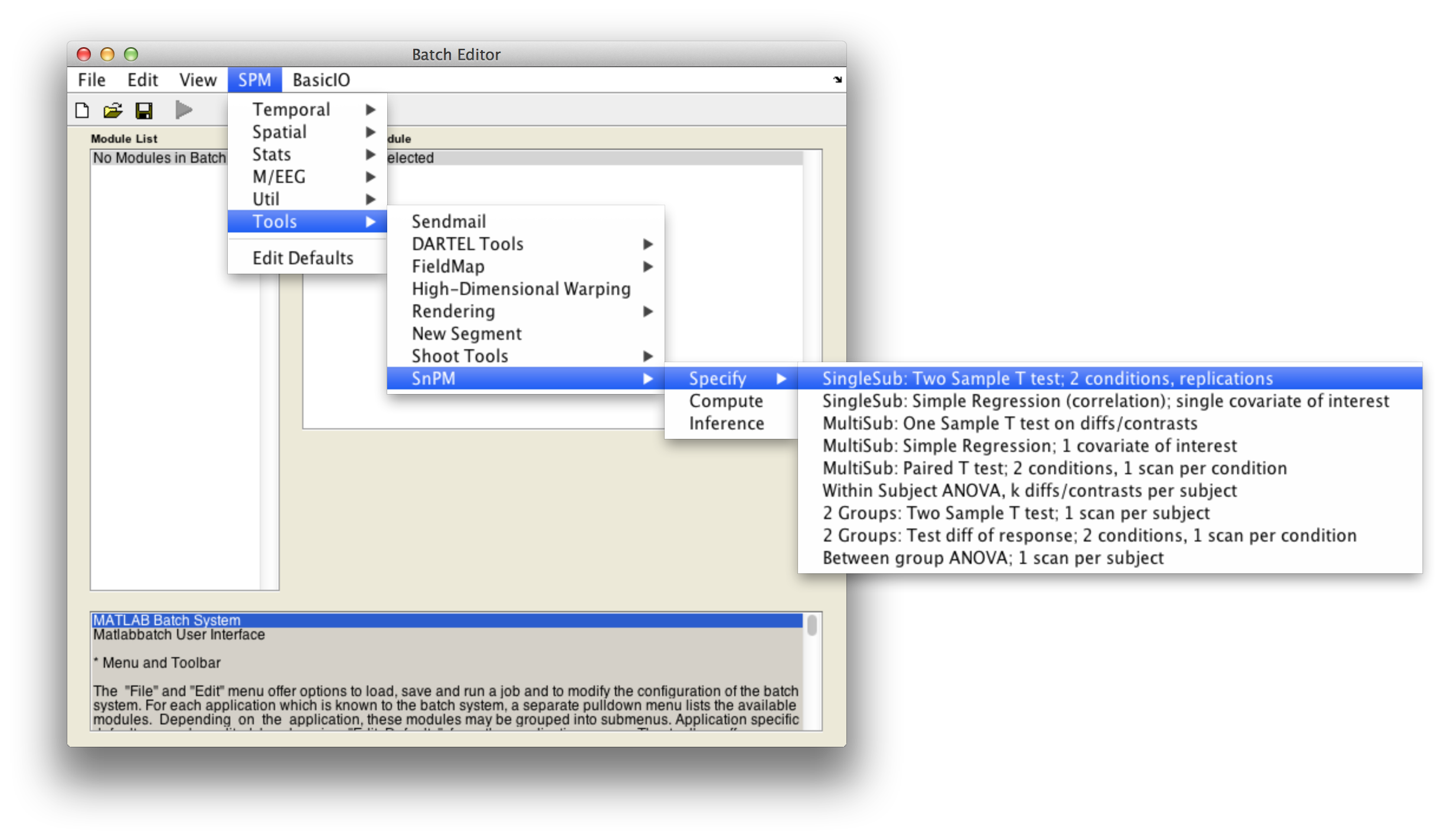
Then fill in the required fields as follows:
Analysis directory: Select the directory in which the analysis files will be stored.Images to analyze: Select all scan files from thePET_motordirectory (i.e.s8np1160em01R.img->s8np1160em12R.img). It is important that you enter them in time order.Replication of conditions:6, as we have 6 repetitions in the motor dataset.Condition index. This is a sequence of 1's and 2's (1's for activation, 2's for baseline) that describe the labeling used in the experiment. Since this experiment was not randomized we have a nice neat arrangement:1 2 1 2 1 2 1 2 1 2 1 2Size of exchangeability block:4. From the discussion above we know we don't want a 12-scan EB, so will use a EB size of 4, since this gives over 200 permutations yet is a small enough EB size to protect against severe temporal confounds. The help text for each SnPM plug in file gives a formula to calculate the number of possible permutations given the design of your data. Use the formula when deciding what size EB you should use.
Cluster inference:Yes (slow, may create huge SnPM_ST.mat file).
Variance smoothing:10 10 10.
Masking,Threshold masking: SelectRelative.Global calculation: SelectMean.Global normalisation,Overall Grand Mean Scaling: SelectYes.Global normalisation,Normalisation: SelectANCOVA.
CovariatesNumber of permutationsMemory usage
Finally, the Batch window is as below:
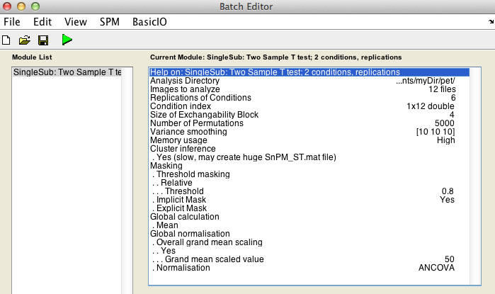
The start button in SPM batch window is now green  , click on it to run the job.
SnPM will now create the file SnPMcfg.mat. and show the Design Matrix in the Graphics window.
Computing the nonParametric permutation distributions
In the SPM menu, under Tools -> SnPM, select Compute.
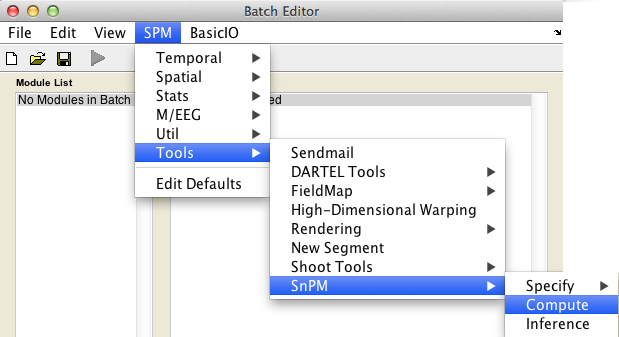
Then fill in the required field as follows:
SnPMcfg.mat configuration file: Select theSnPMcfg.matfile just created.
The start button in SPM batch window is now green  , click on it to run the job.
Results
In the SPM menu, under Tools -> SnPM, select Inference.
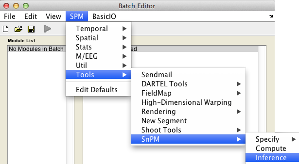
The uncorrected and FWE-corrected p-values are exact, meaning if the null hypothesis is true exactly 5% of the time you'll find a P-value 0.05 or smaller (assuming 0.05 is a possible nonparameteric P-value, as the permutaiton distribution is discrete and all p-values are multiples of 1/nPerm). FDR p-values are valid based on an assumption of positive dependence between voxels; this seems to be a reasonable assumption for image data. Note that SPM's corrected p values derived from the Gaussian random field theory are only approximate.
Voxel-wise inference
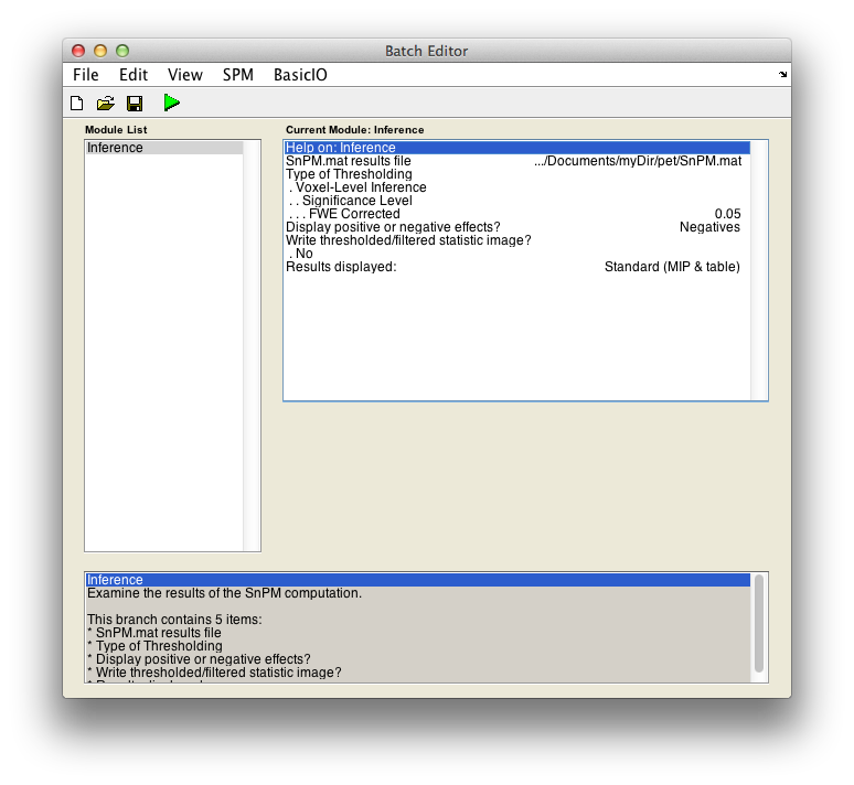
For voxel-wise inference with p < 0.05 FWE corrected, fill in the required field as follows:
SnPM.mat results file: Select theSnPM.matfile just created.Display positive or negative effects?: Positive corresponds to "Condition 2 - Condition 1'' and negative to "Condition 1 - Condition 2''. If you are interested in a two tailed test repeat this whole procedure twice but halve your p value threshold value in the next entry. SelectNegatives
Type of thresholdingResults displayed
Finally, the Batch window is as below:
The start button in SPM batch window is now green  , click on it to run the job.
SnPM will then plot a MIP of those voxels surviving the SnPM critical threshold.

The figure is titled "SnPM{Pseudo-t}"" to remind you that the variance has been smoothed and hence the intensity values listed don't follow a t distribution. The tabular listing indicates that there are 70 voxels significant at the 0.05 level; the maximum pseudo-t is 6.58 and it occurs at (-38, -28, 48).
Cluster-wise inference
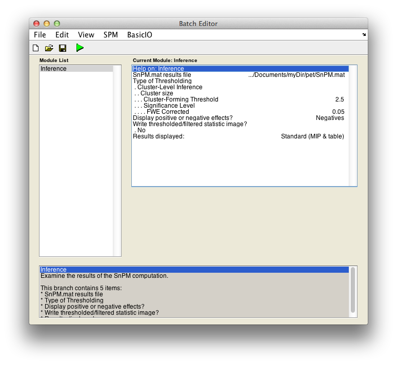
For cluster-wise inference with p < 0.05 FWE corrected using a cluster-forming threshold of pseudo-T > 2.5, fill in the required field as follows:
SnPM.mat results file: Select theSnPM.matfile just created.Type of thresholding: Selectcluster-wise inferenceCluster-forming threshold: Now you have to decide on a threshold. This is a perplexing issue which we don't have good suggestions for right now. Since we are working with the pseudo-t, we can't relate a threshold to a p-value, or we would suggest a threshold corresponding to, say, 0.01.When SnPM saves supra-threshold stats, it saves all pseudo-t values above a given threshold for all permutations. The lower lower limit shown (it is 1.23 for the motor data) is this "data collection" threshold. The upper threshold is the pseudo-t value that corresponds to the corrected p-value threshold (4.98 for our data); there is no sense entering threshold above this value since any voxels above it are already significant by intensity alone.
Trying a couple different thresholds, we found 2.5 to be a good threshold. This, though, is a problem. The inference is strictly only valid when the threshold is specified a priori. If this were a parametric t image (i.e. we had not smoothed the variance) we could specify a univariate p-value which would translate to specify a t threshold; since we are using a pseudo t, we have no parametric distributional results with which to convert a p-value into a pseudo t. The only strictly valid approach is to determine a threshold from one dataset (by fishing with as many thresholds as desired) and then applying that threshold to a different dataset. We are working to come up with guidelines which will assist in the threshold selection process.
Type2.5Display positive or negative effects?: Positive corresponds to "1" - "2" and negative to "2" - "1". If you are interested in a two tailed test repeat this whole procedure twice but halve your p value threshold value in the next entry. SelectNegatives
Results displayed
Finally, the Batch window is as below:
The start button in SPM batch window is now green  , click on it to run the job.
SnPM will then plot a MIP of those voxels surviving the SnPM critical threshold.

Now we see that we have identified one 561 voxel cluster as being significant at 0.005 (all significances must be multiples of 1 over the number of permutations, so this significance is really 1/216=0.0046). This means that when pseudo-t images from all the permutations were thresholded at 2.5, no permutation had a maximum cluster size greater than 561.

