BSGLMM: ManualBayesian Spatial Generalised Linear Mixed ModelBy Tian Ge, Tim Johnson & Tom Nichols |
This page... Introduction Manual Example Download References Contact |
System Requirements
|
Installation
Unpack the archive in a directory of your choice. You will need the latest version of GNU GCC to compile the source code.
In order to compile the code, run the Makefile from inside the extracted directory with
$ make
The executable thereby created is named BinCar.
Source files included in the download
- main.cu
- mcmc.cpp
- covar.cpp
- covarGPU.cu
- read_data.cpp
- cholesky.cpp
- randgen.cpp
- nifti1_read_write.cpp
- accompanying <header_files>
Potential Issues during installation
- Different version of CUDA.
solution: Update the first lines in the Makefile to your CUDA version.
- Shared libraries not found.
solution: Include the following line in your .bashrc file (for CUDA 5.0 in this case):
export LD_LIBRARY_PATH=/usr/local/cuda-5.0/lib64
Running the Code
USAGE
$ ./BinCar NTypes NCov GPU Design Mask WM [MaxIter BurnIn]
To see a short description of all intput arguments, try running the program without any command line arguments:
$ ./BinCar
Input arguments
- NTYPES: number of different types or groups or classes in the data set
- NCOV: total number of covariates (Note: count must include types/groups as dummy covariates)
- GPU: run code on GPU (1) or CPU (0)
Note: We strongly recommend running the code on a GPU. (CPU not testet! Use with caution.)
- DESIGN: Text file, tab or space separated data file that contains all input data.
- MASK: Filename of mask image (must be located in './images' directory); specify '1' to use default (mask.nii.gz).
- WM: Filename of withe matter mask image (must be located in './images' directory): specify '0' to use none and '1' to use default (avg152T1_white.nii.gz)
- MAXITER (optional): Total number of iterations. Defaults to 1,000,000; use fewer for testing to save time.
- BURNIN (optional): Number of burn-in iterations. Defaults to 500,000; try using half the number of MAXITER.
Format of input file DESIGN (e.g. data.dat)
The first row of data.dat specifies the names of the columns (variables). All other rows contain the individual data for each subject.
The first is subject ID, followed by one column for each type/group/class in the data. (E.g. a data set consisting of patients and healthy controls would have two columns of zeros and ones, indicating to which group each subject belongs.)
The next columns specify covariates, one for each covariate. Important note: these covariates need to be mean-centered.
The last column contains the file name of the image for each subject. (Note that the image file does not have a path, all images need to be stored in a subdirectory named "images".)
Here are the first lines of an example data.dat file containing two classes and five additional covariates. (The full file is included in the example data bundle below.)
Image files
- mask.nii.gz: whole-brain mask
- WM_mask.nii.gz (optional): white matter mask. This must be a 8 bit (unsigned char, uint8) image file.
- <image_files.nii.gz>: binary lesion masks for each subject.
NOTE: The program expects a subdirectory named "./images" in the main directory. ALL image files (including the mask and WM files) must be in the *.nii.gz format and stored in this subdirectory.
Other input files
- seed.dat (optional): containing three starting seed numbers for random number generator
Execution from command line - example
This is an example of how to run the code after it has been compiled:
$ <path_to_exe_dir>/BinCar 2 7 1 data.dat 1 0 10000 5000
For this example, input arguments used are:
NTYPES=2; NCOV=7 (i.e. 5 covariates + 2 types); GPU=1; DESIGN=data.dat; MASK=default; WM=none; MAXITER=10,000; BURNIN=5,000.
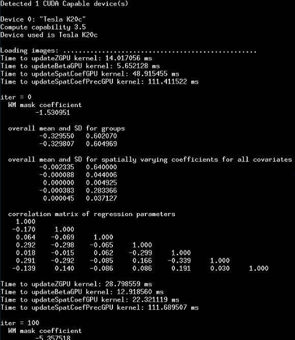
Here is an example screenshot of the terminal output after the first 500 iterations. The first few lines give some info about which GPU's are available and used; followed by diagnostic output for every 100 iterations:
Output files
Terminal output during runtime
By default only the current number of completed iterations of the MCMC algorithm is displayed. Additional information (e.g. current parameter values, GPU times to compute parameter updates, etc.) can be displayed by un-commenting the respective lines in the source files (mostly found in mcmc.cpp).
Output files
File structure of Qhat.dat and Qhat2.dat:
| ID | prob type1 | prob type2 | [additional classes] |
predicted type | true type |
| 0 | 0.9999 | 0.0001 | ... | 0 | 0 |
| 1 | 0.9999 | 0.0001 | ... | 0 | 0 |
| 2 | 0.0000 | 1.0000 | ... | 1 | 1 |
| ... | ... | ... | ... | ... | ... |
The 1st column contains a running count for all subjects (starting from zero). The 2nd, 3rd, 4th, etc. columns (depending on the total number of types) give the predicted probabilities for each type. Most interesting is the second-to-last column which provides a prediction of each subject into one of the given types. For reference and comparison, the last column displays the true type as given in the input data.
Results
Posterior mean probabilities for each type/group/class of data are given in the files prb_<NAME_OF_TYPE>.nii.
The probability maps for spatial and standardised spatial coefficients can be found in spatCoef_<NAME_OF_COVAR>.nii and standCoef_<NAME_OF_COVAR>.nii respectively.
Qhat.dat and Qhat2.dat provide raw data for prediction and classification accuracy using an importance sampling approach (see Sec. 4.2 in the paper). For example, the total prediction accuracy for a given data set is simply the number of correctly classified subjects (predicted type == true type) divided by the total number of subjejcts.
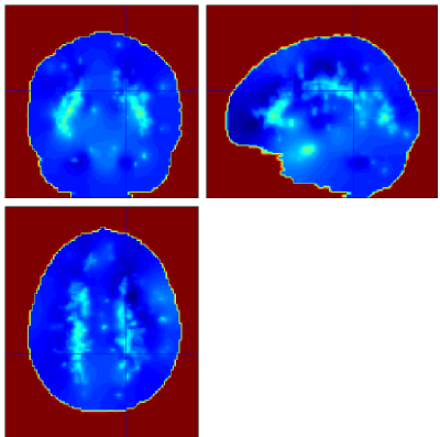
Example Output
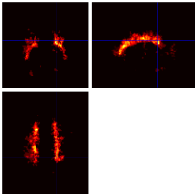
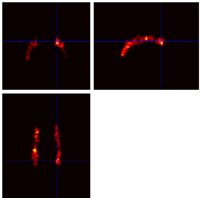
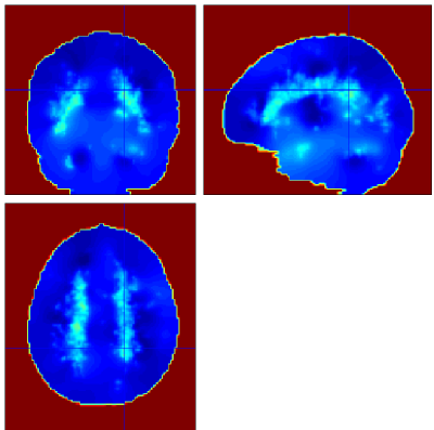
Below are example slices of some of the generated output files for the same slice position (voxel 34.6 40.1 50.9)
Convergence Diagnostics
MCMC algorithms need to be monitored for convergence. Since saving the chains for all parameters, i.e. voxels, is infeasible we recommend monitoring a group of (say 10) voxels in qualitatively different regions (e.g. regions with both high and low lesion load).
For details please see Sec. 4.4 in the paper.
Example Data
Download example data here ( demo-data) and extract the archive in a directory of your choice.
This dataset contains binary lesion data from 50 subjects (binLesionData_<subject_ID>.nii.gz) with multiple sclerosis. The subjects are categorised into two disease subtypes (25 relapsing-remitting MS, 25 secondary progressive MS).
The DESIGN file is called data_demo.dat and includes the following five demographic and clinical covariates: sex, age, disease duration, EDSS score, PASAT score.
Additionally, a whole-brain mask (mask.nii.gz) and a white matter mask (avg152T1_white.nii.gz) are provided.
Example Classification Results
As both groups contain the same number of subjects, there is no difference between uniform and empirical priors and thus Qhat.dat and Qhat2.dat give the same results. For this data set prediction accuracy for classification into one of the two types is very high (98%) with only one subject (subj ID 1013) misclassified.